#Load package
library("mgrtibbles")
#Set seed for random sampling
set.seed("483")
#mushroom_tbl tibble for demonstration
mushroom_tbl <- mgrtibbles::mushroom_tbl |>
    #Random sample of 150 rows
    dplyr::slice_sample(n = 150, replace=FALSE)
#Reset random seed to normal operation
set.seed(NULL)Labels

The column/variable names in a tibble are used to specify the various aesthetics. By default these names are used as the labels of the specified aesthetics (e.g. x and y labels).
However, what makes a good column/variable name does not always make a good label. The column/variable names we use in these materials have underscores (_) and are all uncapitalised (e.g. mushroom_tbl). For our labels we want spaces instead of underscores and we want some capitalisation.
To specify our aesthetic labels we will use the component labs().
Dataset
We’ll recreate many of the plots in the geom_point() chapter, so we’ll load the mushroom_tbl data from the mgrtibbles package (hyperlink includes install instructions). We will extract a random sample of 150 rows with slice_sample().
Axes labels
The most common labels to add to a ggplot are the x and y labels.
Create the default scatter plot. We’ll specify the x and y labels in the ggplot2::lab() function with x=, and y=.
mushroom_tbl |>
    ggplot2::ggplot(aes(x = stem_width, y = stem_height)) +
    ggplot2::geom_point() +
    ggplot2::labs(x = "Stem width", y = "Stem height")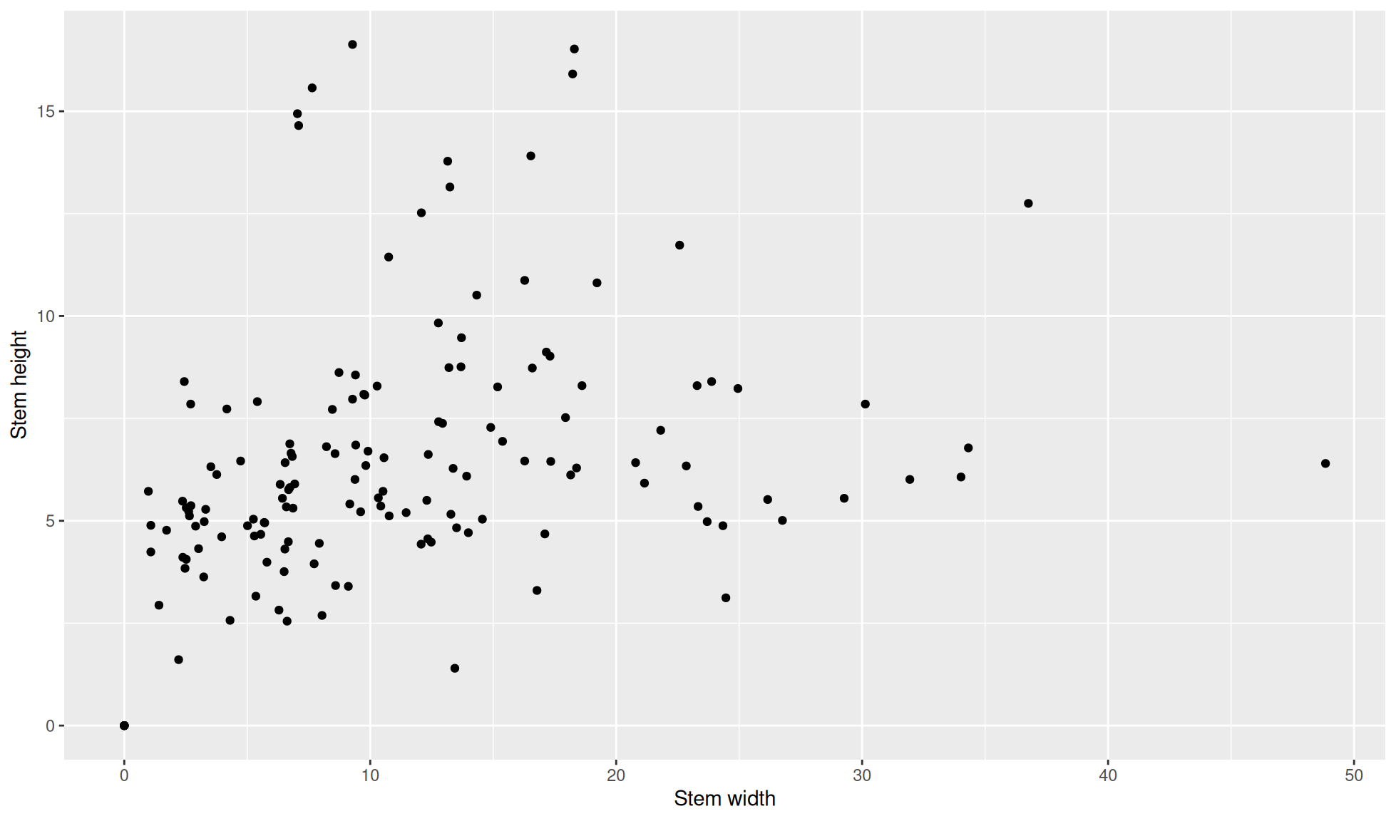
Legend labels
When some aesthetics are added a corresponding legend is added to the plot. We can change the labels of these legends with ggplot2::labs().
Create the scatter plot with colour & shape groups. Assign label names for the x, y, shape, and colour aesthetics.
mushroom_tbl |>
    ggplot2::ggplot(aes(x = stem_width, y = stem_height,
                        shape = class, colour = cap_shape)) +
    ggplot2::geom_point(size = 2) +
    ggplot2::labs(x = "Stem width", y = "Stem height",
                    shape = "Class", colour = "Cap shape")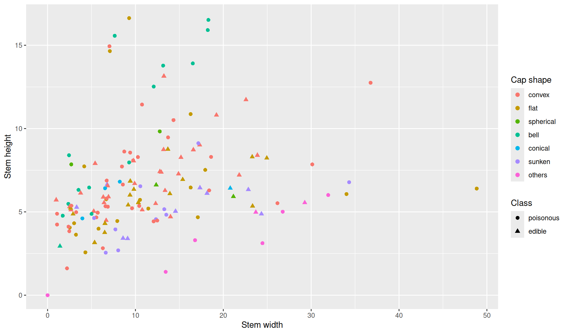
Title
Two other useful labels to add to a plot is the title and sub title.
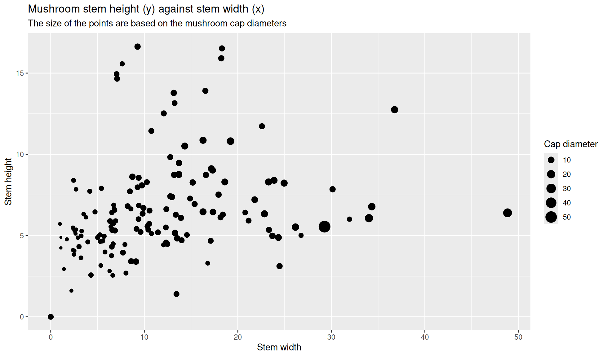
Create the Scatter plot with points sized by a continuous variable. This time we’ll include a title (title=) and sub title (subtitle=), as well as setting the size legend with size= in the ggplot2::labs() function.
mushroom_tbl |>
    ggplot2::ggplot(aes(x = stem_width, y = stem_height, size = cap_diameter)) +
    ggplot2::geom_point() +
    ggplot2::labs(x = "Stem width", y = "Stem height", size = "Cap diameter",
                    title = "Mushroom stem height (y) against stem width (x)",
                    subtitle = "Size of points based on mushroom cap diameters")