Geom bar

Bar charts are commonly used to display the counts of different categorical values.

In this page we will create bar charts with ggplot2::geom_bar(). Through examples we will demonstrate creating:

The default bar chart
A flipped bar chart
A stacked bar chart using a second categorical variable
A side-by-side bar chart using a second categorical variable
A relative proportion bar chart

Dataset

For demonstration we’ll load the amphibian_div_tbl data from the mgrtibbles package (hyperlink includes install instructions). Additionally, we’ll select the columns “iucn_2cat”, “Order”, and “Family” which we will use for plotting. Then we’ll remove any rows with an NA value using tidyr::drop_na.

amphibian_div_tbl details

#Library
library("mgrtibbles")
#Data
amphibian_div_tbl <- 
    mgrtibbles::amphibian_div_tbl |>
    #Select to retain only the iucn_2cat and Order columns
    dplyr::select(iucn_2cat,Order,Family) |>
    #Drop any rows with an NA
    tidyr::drop_na()

Default bar chart

When creating a bar chart with ggplot2::geom_bar() a categorical variable/column can be mapped to the x aesthetic. The function will then calculate the count numbers.

Create a bar chart of the iucn_2cat variable/column. This is a column of categorical factors (<fct>) representing IUCN categories of:

LC: Least Concern
nonLC: non Least Concern including Near Threatened, Vulnerable, and Endangered

amphibian_div_tbl |>    
    ggplot2::ggplot(aes(x = iucn_2cat)) +
        ggplot2::geom_bar()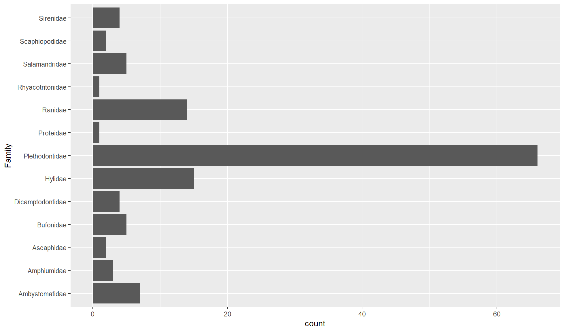

Flipped bar chart

If there are a lot of unique values in the categorical variable you can map it to the y aesthetic to create a flipped bar chart. This is especially useful if the values have long names that would struggle to fit as labels side by side on the x-axis.

Create a flipped bar chart of the Family categorical character variable/column.

amphibian_div_tbl |>    
    ggplot2::ggplot(aes(y = Family)) +
        ggplot2::geom_bar()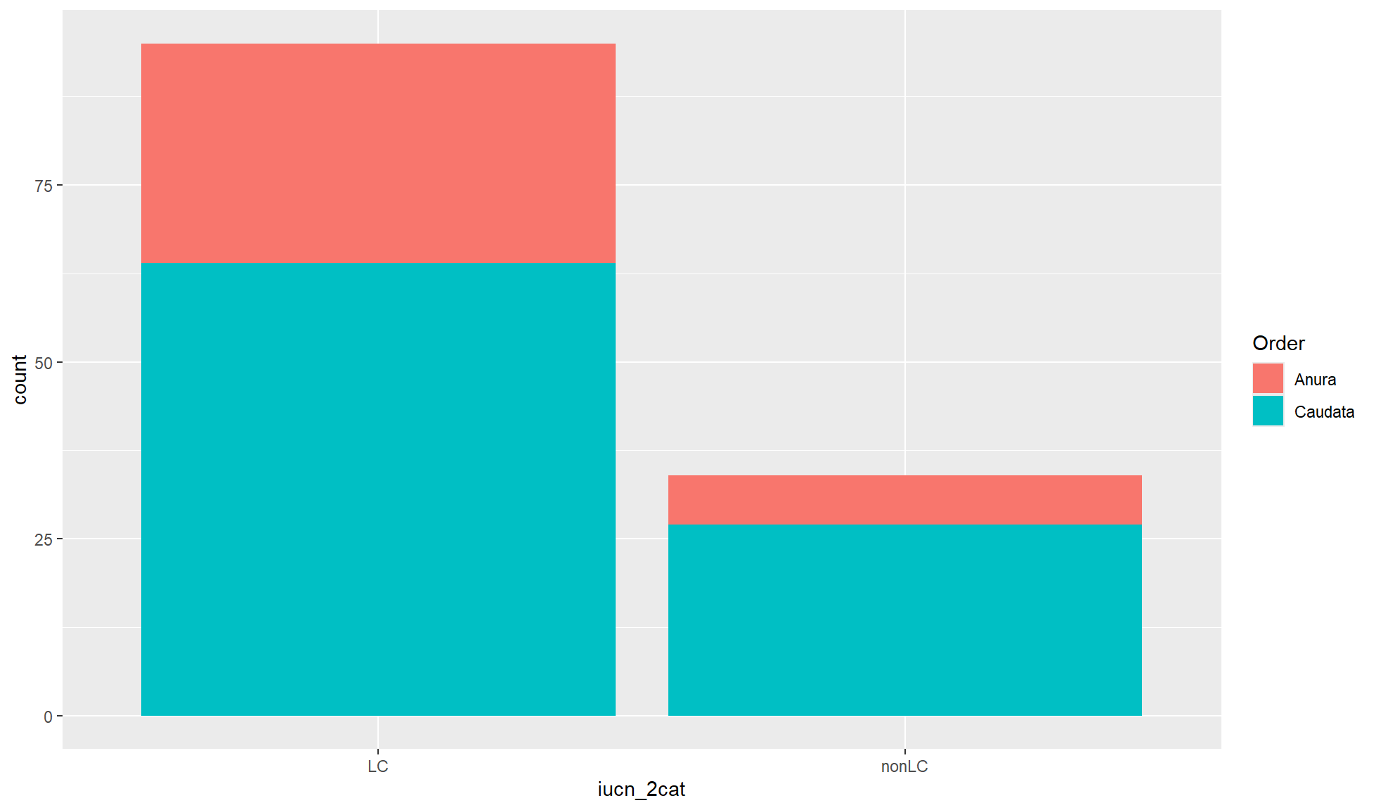

Stacked bar chart

It is common to map a second categorical variable/column to the fill aesthetic. By default this will create a stacked bar chart where the fill variable is represented by colours filling the bar chart. This is useful is you are more interested in the differences between the x-axis groupings.

Create a stacked bar chart of “iucn_2cat” counts where the fill of the bar chart is coloured by “Order”.

amphibian_div_tbl |>    
    ggplot2::ggplot(aes(x = iucn_2cat, fill = Order)) +
        ggplot2::geom_bar()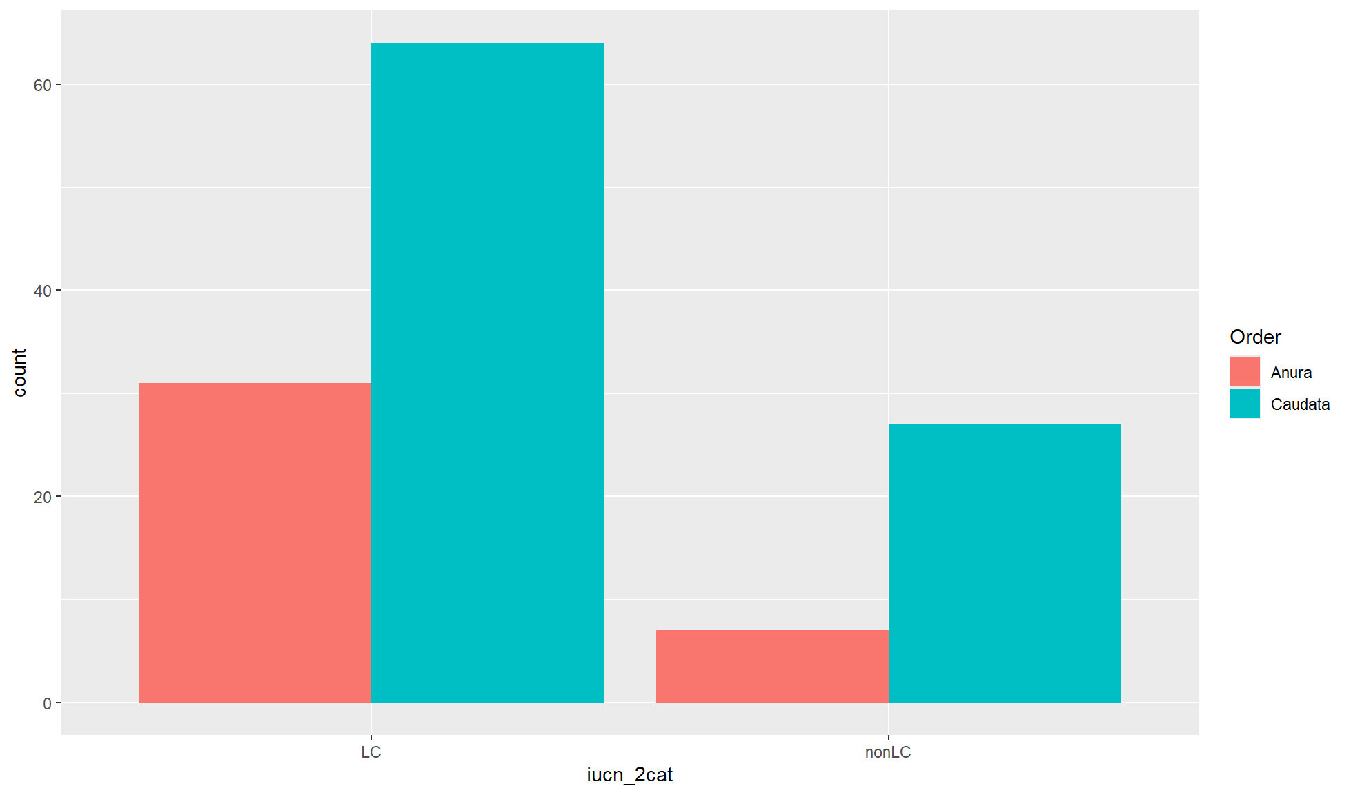

Side-by-side bar chart

When you are interested in the differences within the x-axis groupings you can created a side-by-side bar chart. This is carried out by using the position= option in ggplot2::geom_bar() and setting it to "dodge".

Create a side-by-side bar chart of “iucn_2cat” counts where the fill of the bar chart is coloured by “Order”.

amphibian_div_tbl |>    
    ggplot2::ggplot(aes(x = iucn_2cat, fill = Order)) +
        ggplot2::geom_bar(position = "dodge")

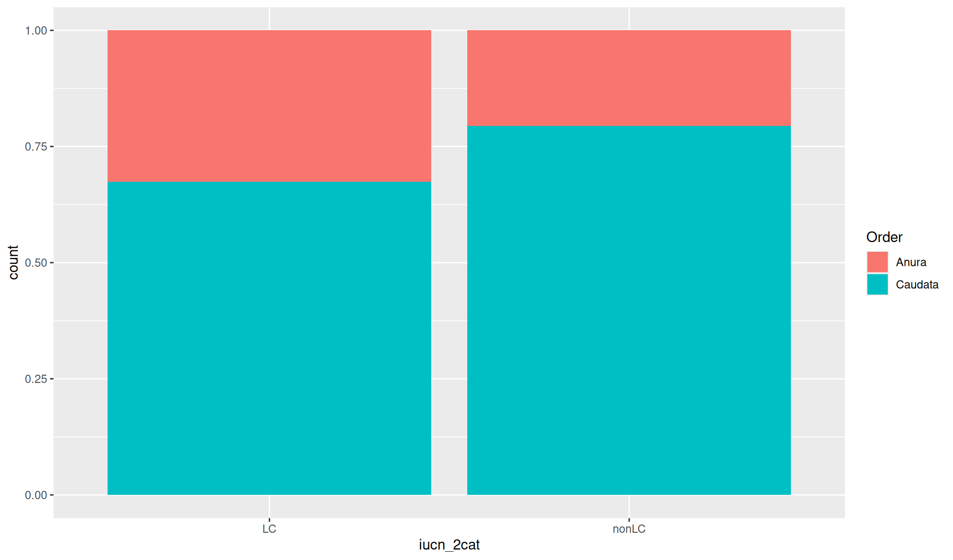
Relative proportion bar chart

ALthough absolute count values are useful for bar charts you will sometimes want relative proportions. To convert the values so the total x-axis count per group equals 1 you can set position= to "fill".

Create a relative proportion bar chart of “iucn_2cat” counts where the fill of the bar chart is coloured by “Order”.

amphibian_div_tbl |>    
    ggplot2::ggplot(aes(x = iucn_2cat, fill = Order)) +
        ggplot2::geom_bar(position = "fill")