#Load package
library("mgrtibbles")
#Set seed for random sampling
set.seed("483")
#mushroom_tbl tibble for demonstration
mushroom_tbl <- mgrtibbles::mushroom_tbl |>
    #Random sample of 150 rows
    dplyr::slice_sample(n = 300, replace=FALSE)
#Reset random seed to normal operation
set.seed(NULL)Facetting
Facetting splits a plot into multiple panels using one or two metadata variables. This allows you to separate groups so you can more easily see the differences within and between the groups.
Dataset
We’ll create scatter plots similar to those in the geom_point() chapter, so we’ll load the mushroom_tbl data from the mgrtibbles package (hyperlink includes install instructions). We will extract a random sample of 300 rows with slice_sample().
Facet grid
The function ggplot2::facet_grid() allows you to split/facet a plot by columns and rows. This can be used if you have one or two discrete variables you want to facet by.
It is important to note that with this method the scales are fixed (i.e. all the panels have the same scale) by default. To learn more and edit this see the facet scales section.
facet_grid() reference webpage
Facet grid by columns
Create a scatter plot of stem_height (y) against stem_width (x).
We’ll facet the data by the variable class, facetting by columns with dplyr::facet_grid(cols = dplyr::vars(class)).
Note: We have to place the variable/column name into the dplyr::vars() function for this.
mushroom_tbl |>
    ggplot2::ggplot(aes(x = stem_width, y = stem_height)) +
    ggplot2::geom_point() +
    #Facet grid class by columns
    ggplot2::facet_grid(cols = dplyr::vars(class))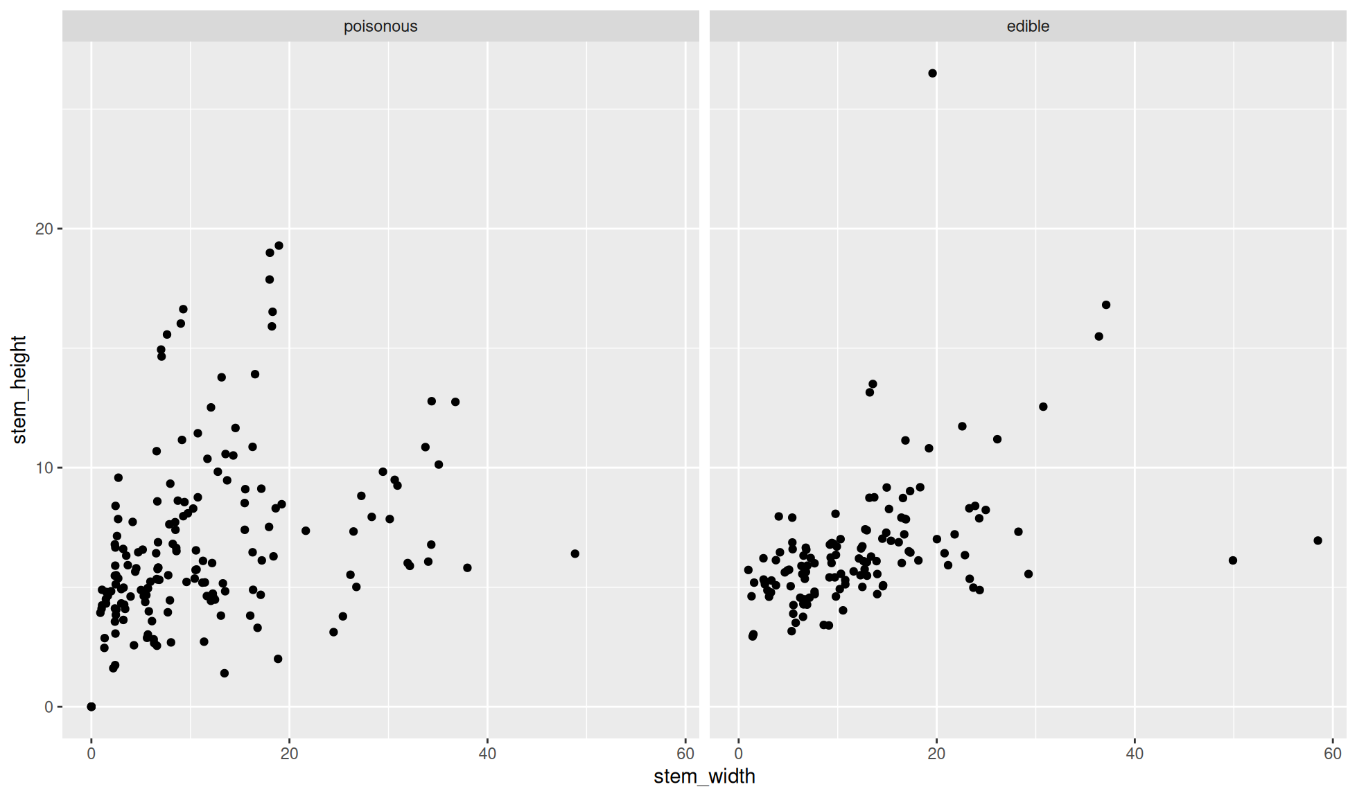
Facet grid by rows
Create a scatter plot of stem_height (y) against stem_width (x).
We’ll facet the data by the variable cap_color, facetting by rows with ggplot2::facet_grid(rows = dplyr::vars(cap_color)).
Note: We have to place the variable/column name into the dplyr::vars() function for this.
mushroom_tbl |>
    ggplot2::ggplot(aes(x = stem_width, y = stem_height)) +
    ggplot2::geom_point() +
    #Facet grid cap_color by rows
    ggplot2::facet_grid(rows = dplyr::vars(cap_color))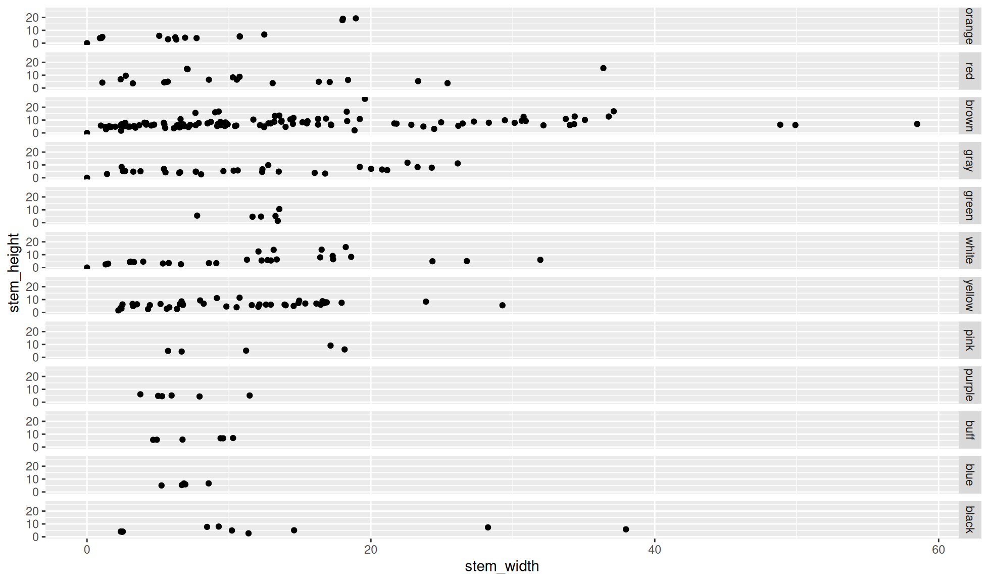
Facet grid by columns and rows
We’ll combine the column and row facetting of the 2 above plots into one plot.
mushroom_tbl |>
    ggplot2::ggplot(aes(x = stem_width, y = stem_height)) +
    ggplot2::geom_point() +
    #Facet grid class by columns and cap_color by rows
    ggplot2::facet_grid(cols = dplyr::vars(class), rows = dplyr::vars(cap_color))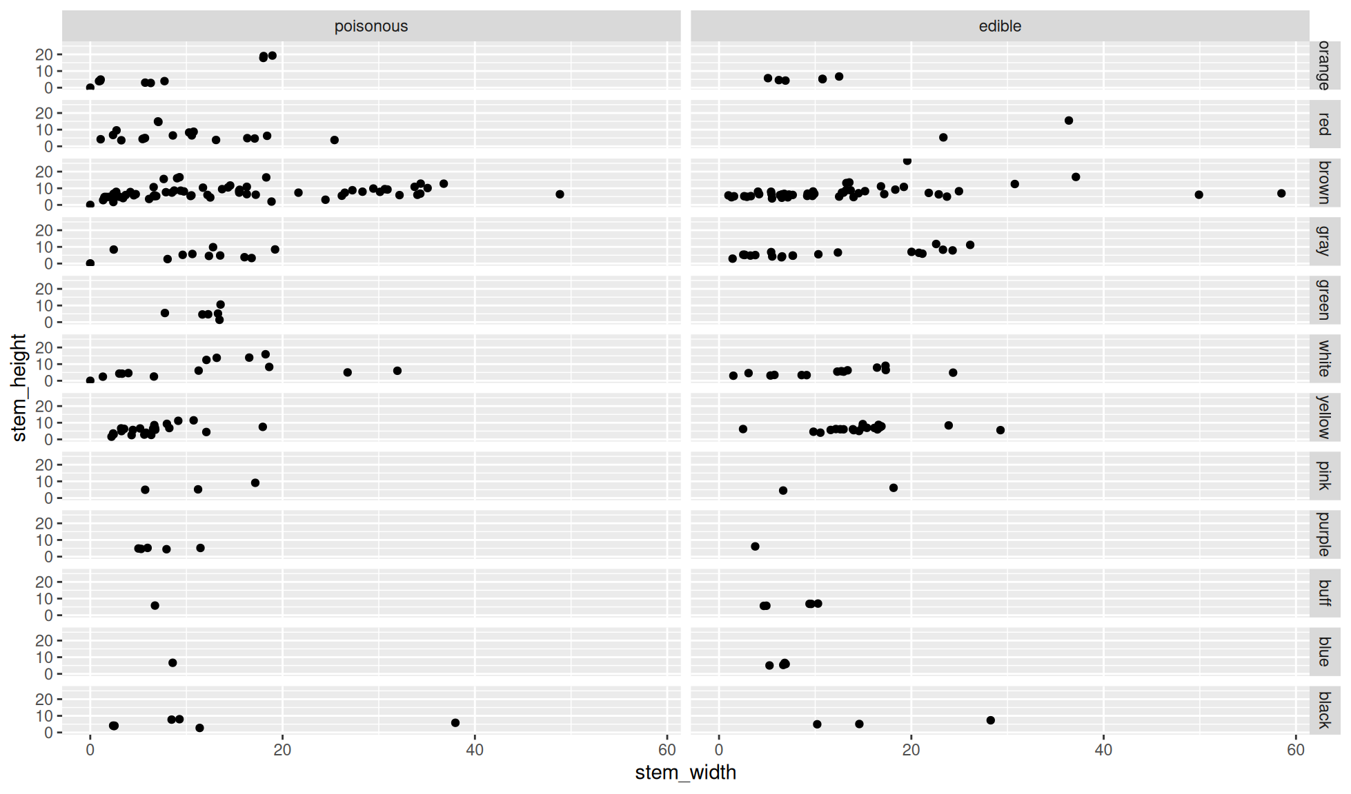
Facet wrap
The function ggplot2::facet_wrap() will wrap panels over multiple rows and/or columns. The number of rows/columns to wrap around can be set with nrow=/ncol=. This is the preferred method when you are facetting by one discrete variable.
It is important to note that with this method the scales are fixed (i.e. all the panels have the same scale). To learn more and edit this see the facet scales section.
facet_wrap() reference webpage
Default facet wrap
Create a scatter plot of stem_height (y) against stem_width (x).
We’ll facet the data by the variable cap_color. This will be carried out with ggplot2::facet_wrap(dplyr::vars(cap_color)).
Note: We have to place the variable/column name into the dplyr::vars() function for this.
mushroom_tbl |>
    ggplot2::ggplot(aes(x = stem_width, y = stem_height)) +
    ggplot2::geom_point() +
    #Facet wrap cap_color
    ggplot2::facet_wrap(dplyr::vars(cap_color))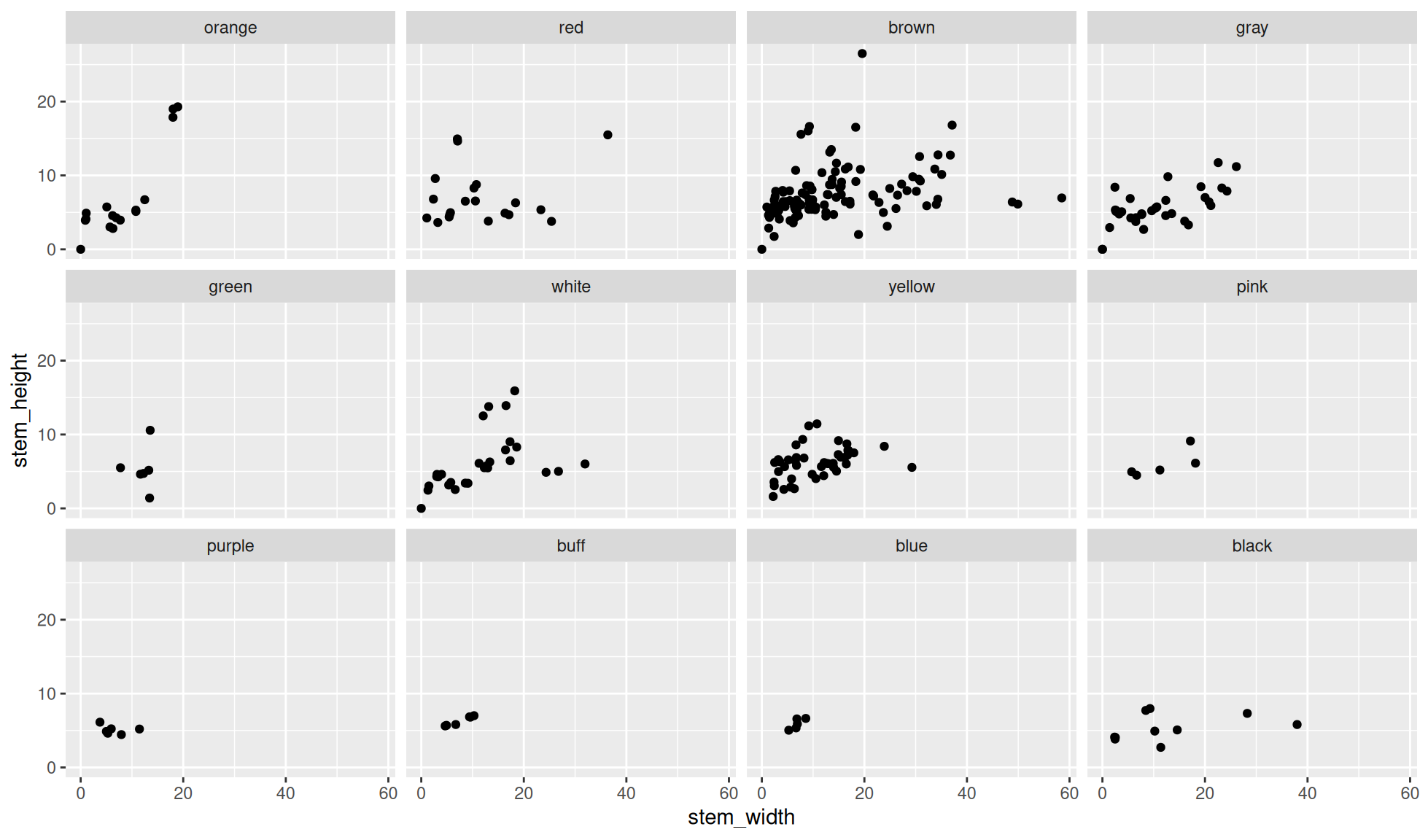
Facet wrap with number of columns
The number of columns to wrap the panels around can be chosen with the ncol= option.
Create a scatter plot of stem_height (y) against stem_width (x).
We’ll facet the data by the variable cap_color. Additionally, we’ll set the number of columns to wrap the panels around to 2 with ncol=2.
mushroom_tbl |>
    ggplot2::ggplot(aes(x = stem_width, y = stem_height)) +
    ggplot2::geom_point() +
    #Facet wrap cap_color with 2 wrapping columns
    ggplot2::facet_wrap(dplyr::vars(cap_color), ncol=2)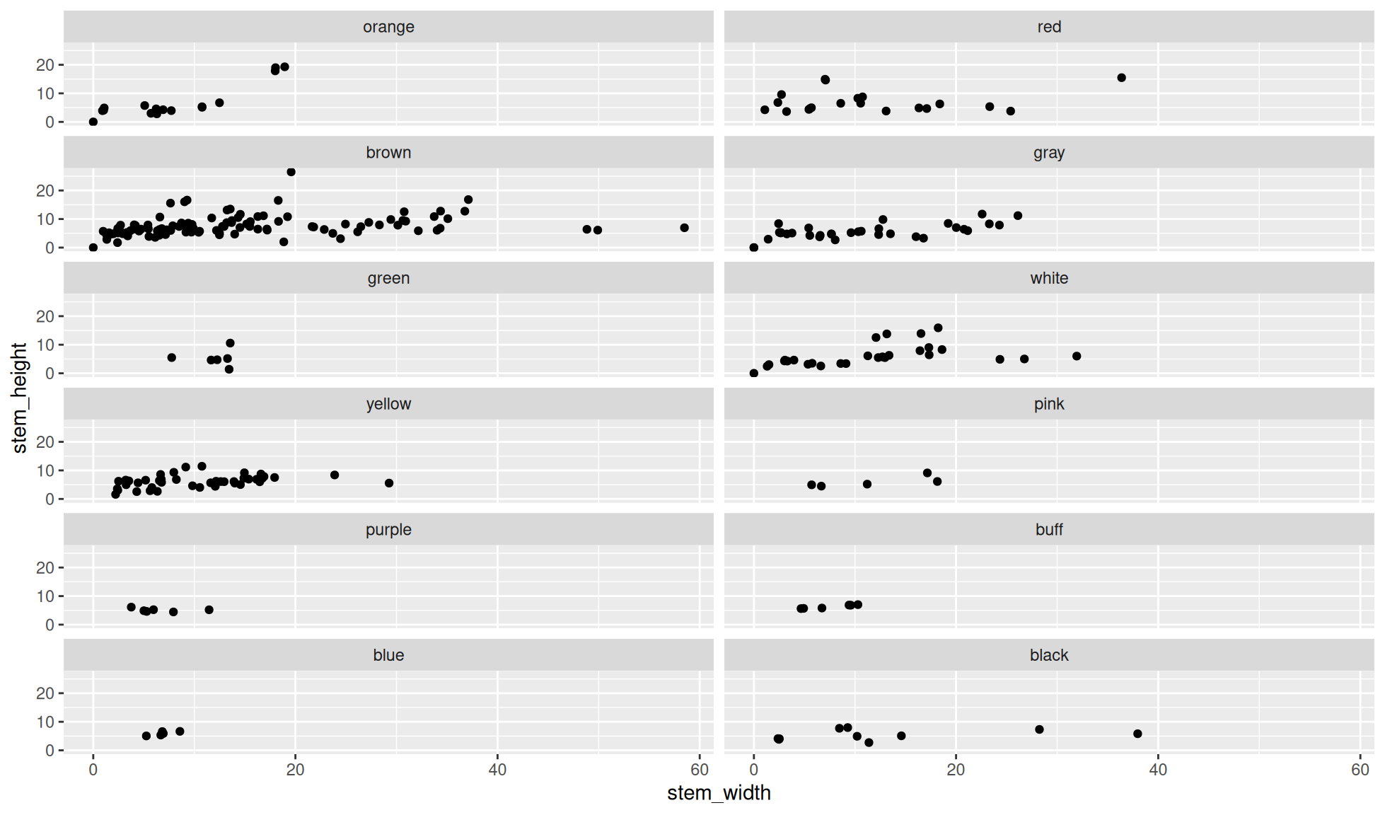
Facet wrap with number of rows
The number of rows to wrap the panels around can be chosen with the nrow= option.
Create a scatter plot of stem_height (y) against stem_width (x).
We’ll facet the data by the variable cap_color. Additionally, we’ll set the number of rows to wrap the panels around to 2 with nrow=2
mushroom_tbl |>
    ggplot2::ggplot(aes(x = stem_width, y = stem_height)) +
    ggplot2::geom_point() +
    #Facet wrap cap_color with 2 wrapping rows
    ggplot2::facet_wrap(dplyr::vars(cap_color), nrow=2)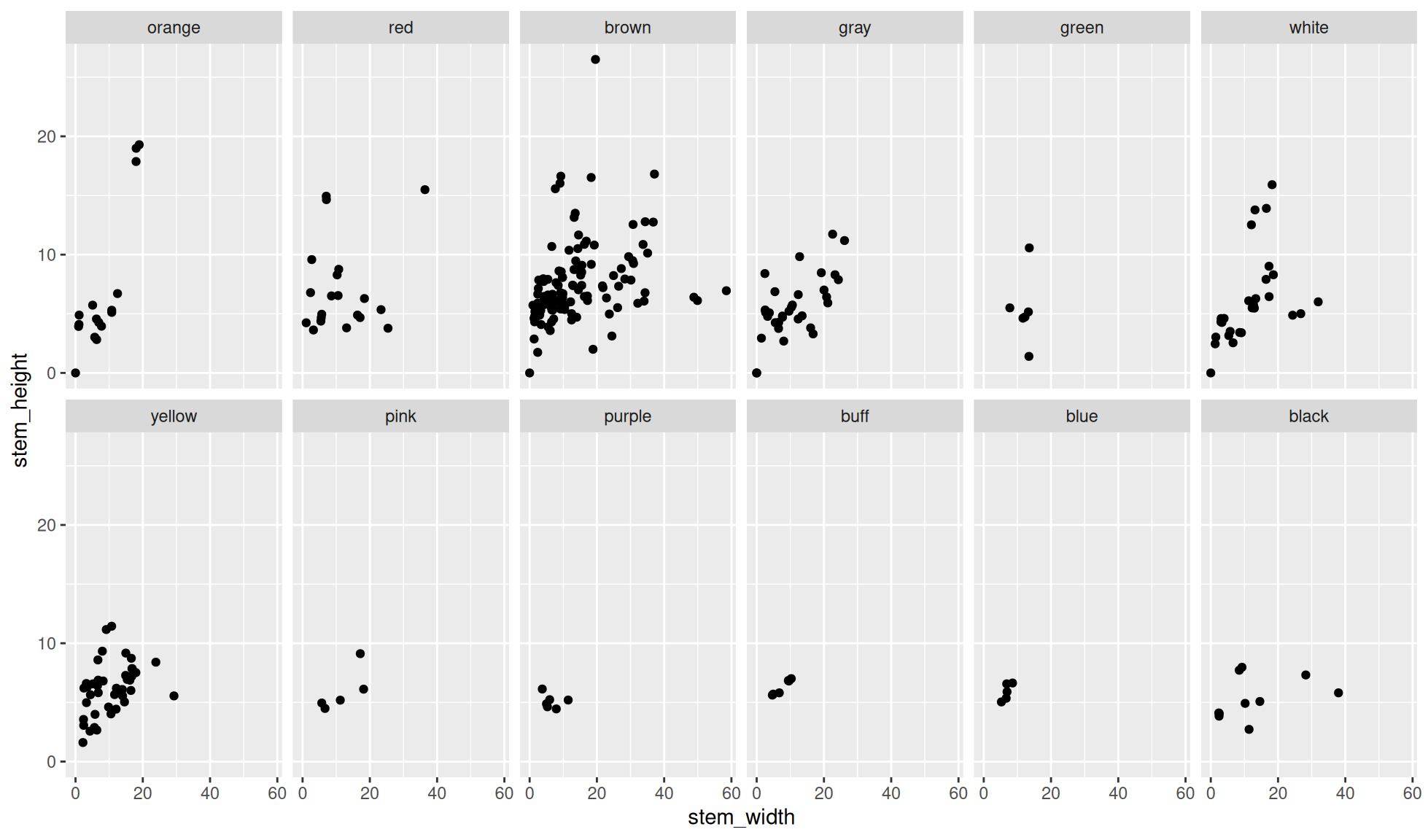
Facet scales
By default both ggplot2::facet_wrap() and ggplot2::facet_grid() will have their scales be “fixed”. This means that the scales will be the same for each panel. In other words the panels in the same row share the same scales which are identical across the columns. This also means the panels in the same column share the same scales which are identical across the rows.
Having the scales as “fixed” allows you to visualise the difference between the different facetting variables. However, this can make it difficult to view the difference within a panel. This can be seen in the above plots with the colour_cap variables: pink, purple, buff, green, and blue. In these variables the points are very close together (overclustered) so it is hard to differentiate between the points.
To change the scales we can use the options scales= with one of the following:
"fixed": This is the default with both scales being fixed"free": This allows both axes scales to be free"free_x": The x axis scale is free but the y axis scale is fixed"free_y": The y axis scale is free but the x axis scale is fixed
Free scales for facet_grid()
Create the same plot as that made in the facet grid by columns and rows and set the scales to free. This is carried out with the option scales="free" within the function ggplot2::facet_grid().
In the below plot notice that the scales for each row and each column are “free”. In other words the scales have been chosen to fit the data in each row and in each column. It is important to note that the scales for each panel are not free.
mushroom_tbl |>
    ggplot2::ggplot(aes(x = stem_width, y = stem_height)) +
    ggplot2::geom_point() +
    #Facet grid class by columns and cap_color by rows
    #Set scales to free
    ggplot2::facet_grid(cols = dplyr::vars(class), rows = dplyr::vars(cap_color),
                        scales="free")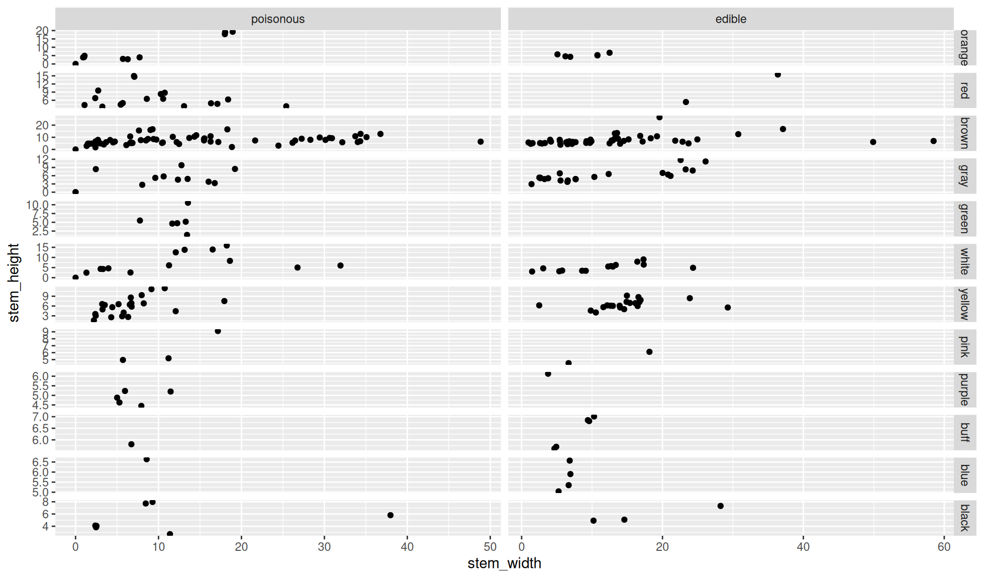
Free scales for facet_wrap()
Create the same plot as that made in the Default facet wrap and set the scales to free. This is carried out with the option scales="free" within the function facet_wrap().
In the below plot notice that the scales for each panel are “free”. In other words the scale have been chosen to fit the data in each panel.
mushroom_tbl |>
    ggplot2::ggplot(aes(x = stem_width, y = stem_height)) +
    ggplot2::geom_point() +
    #Facet wrap cap_color
    ggplot2::facet_wrap(dplyr::vars(cap_color), scales="free")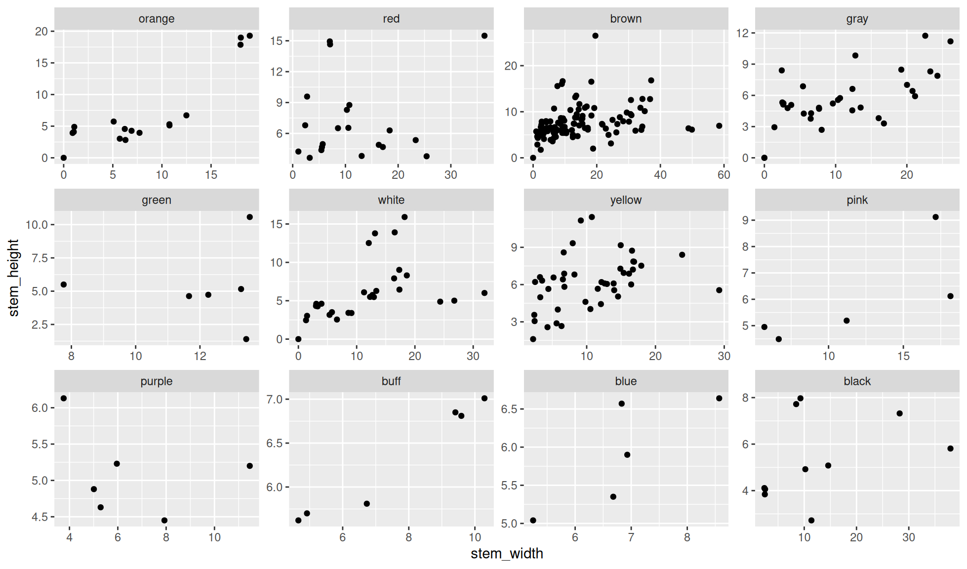
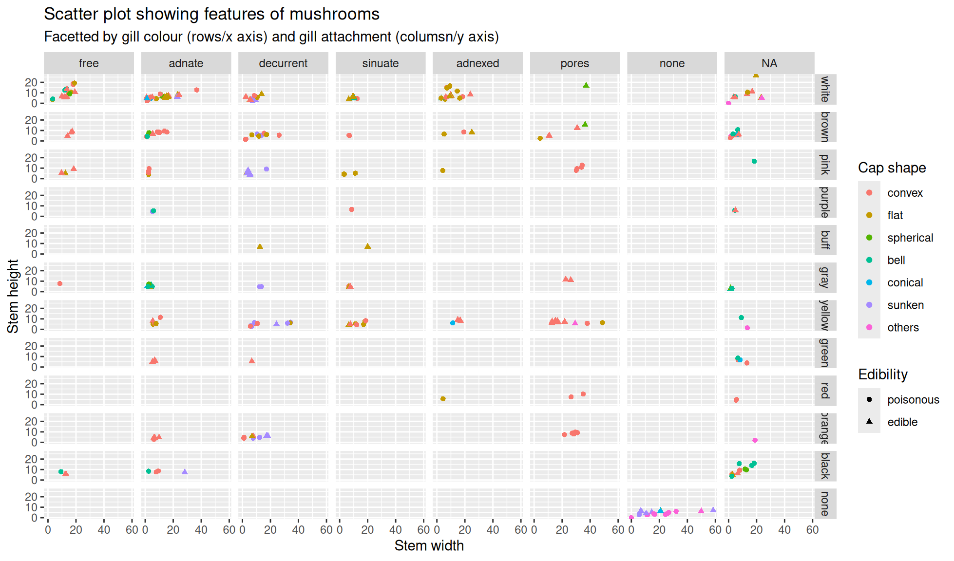
Facets as an aesthetic
Facets become especially useful when you have a lot of variables you would like to represent as aesthetics. There are no limits to the the number of facets you can use, unlike colours and shapes.
Let’s create a final scatter plot plot with the mushroom_tbl tibble. The aesthetics we will set are:
x=stem_widthy=stem_heightcolour=cap_shapeshape=class
Additionally, we will facet with gill_attachment and gill_color.
mushroom_tbl |>
    ggplot2::ggplot(aes(x=stem_width,y=stem_height,color=cap_shape,shape=class)) +
        ggplot2::geom_point() +
        #Facet grid class by columns and cap_color by rows
        ggplot2::facet_grid(
            cols = dplyr::vars(gill_attachment), rows = dplyr::vars(gill_color)) +
        #Labels
        ggplot2::labs(
            title="Scatter plot showing features of mushrooms",
            subtitle="Facetted by gill colour (rows) and gill attachment (columns)",
            x = "Stem width", y = "Stem height",
            color = "Cap shape", shape = "Edibility")