Chapter 23 Bin quality
CoCoPyE is a useful tool to assess the quality of assembled microbial genomes.
This can be used on assemblies produced from single cell, single isolate, or metagenome data.
23.1 Workflow concept
The tool utilises protein domain families from the Pfam database. A protein domain is a region of a protein that folds independently from the rest of the protein. They vary in length from ~50-250 amino acids. Many proteins consist of several domains and a domain can appear in many different proteins.
CoCoPyE estimates quality of a genome by estimating completeness and contamination through an input-preprocessing step followed by a two stage prediction step.
Below is the workflow as a diagram followed by some quick information on how it works. For full details please see the CoCoPyE publication: https://academic.oup.com/gigascience/article/doi/10.1093/gigascience/giae079/7841111
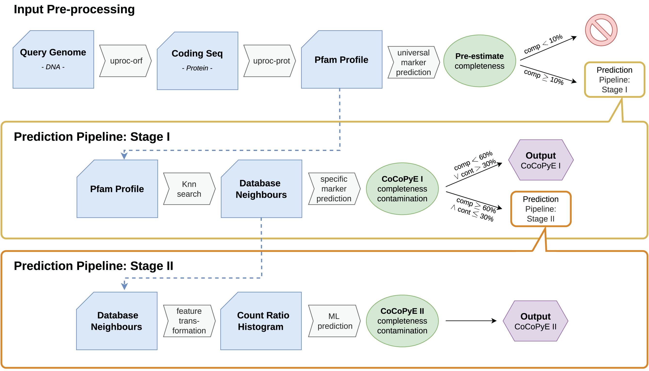
23.1.1 Input Pre-processing
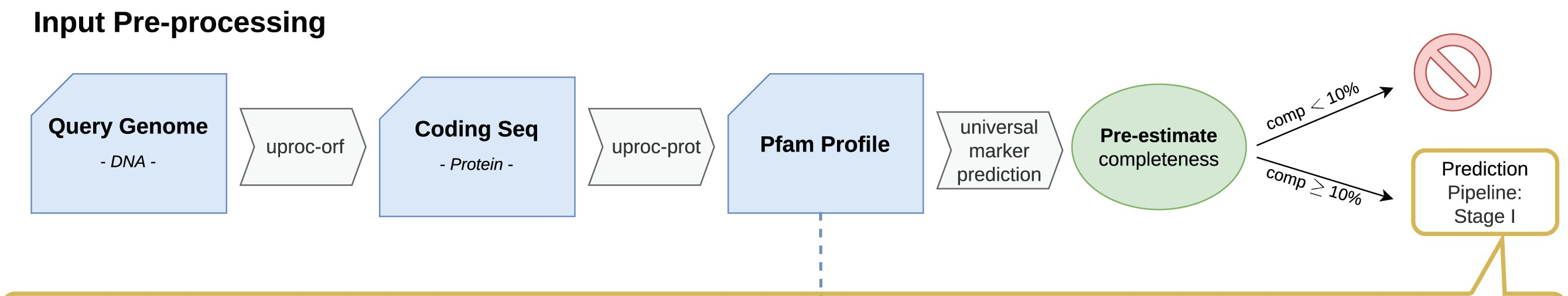
A protein domain search is carried out on all translated open reading frames of our our query genomes, MAGs/bins in our case. The Pfam protein database is used and the tool produces protein domain counts for our query genomes.
The completeness of the query genome is estimated based on one of 2 universal marker sets. The universal marker sets contain the protein domains found in either all reference bacterial genomes or all reference archaeal genomes. Query genomes (MAGS/bins) with a completeness score <10% are rejected and removed from further analysis.
23.1.2 Stage I
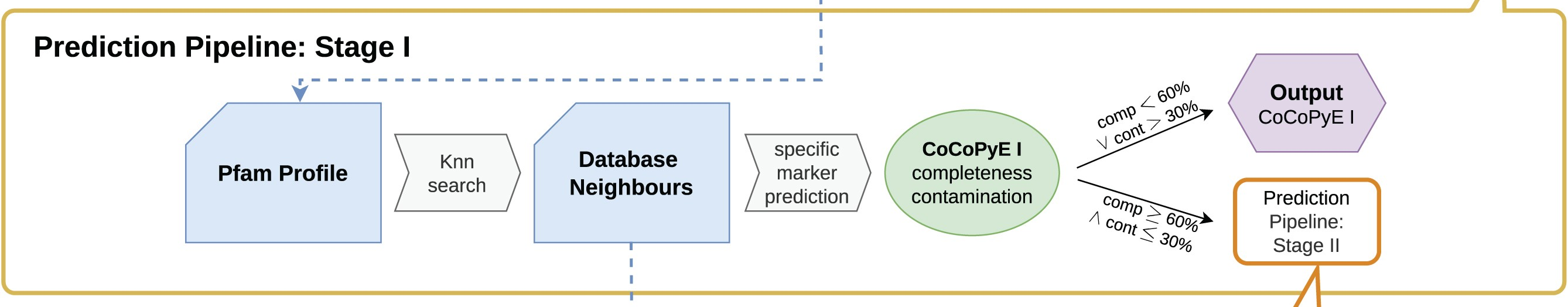
In Stage I the nearest neighbours of our query's protein domains are searched for in the Pfam database. This creates a list of reference protein domains for our query.
Next a specific marker prediction is carried out to create the stage I (i.e. marker based) completeness & contamination values. The Pfam database has information on which taxa these domains are present in. Therefore, sets of domains can be used as markers for specific lineages.
Prediction example
Let's go through a fictional example where we have 26 protein domains PDA-Z which cover 2 different lineages: Gigabacteria and Birthobacteria.
- Both Gigabacteria and Birthobacteria contain domains PDA-F
- Domains PDG-P are only present in Gigabacteria
- Domains PDQ-Z are only present in Birthobacteria
Analysis finds that our query genome contains the domain families PDD-R. We therefore acquire the below results:
- The query genome is classified as belonging to the Gigabacteria lineage as it contains many (in this case all) the domains unique to Gigabacteria (PDG-P) and many of the domains shared by both bacteria.
- Completeness: 81.25%
- It is missing 3 of the domains found in Gigabacteria (PDA-C) 13/16 = 0.8125 = 81.25%
- Contamination: 13.33%
- Of the 15 domains our query has 2 of them do not belong to it in the reference (PDQ & PDR) 2/15 = 0.1333 = 13.33%.
23.1.3 Stage II
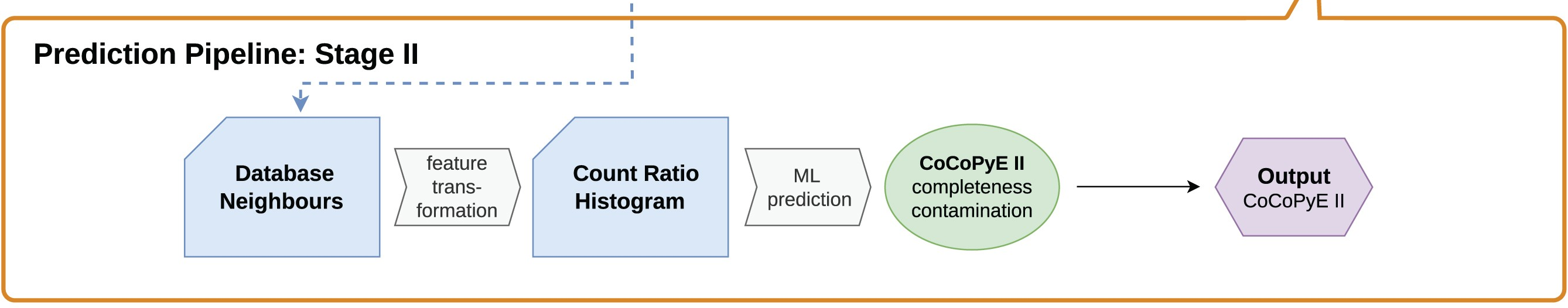
The next step utilises the domain database neighbours found in stage I. With this it creates a count ratio histogram (CRH) to use for a machine learning (ML)/neural network approach. This is carried out to reduce the dimensionality of the data to improve iterative training and reduce the risk of overfitting. But what is a CRH?
Count Ratio Histogram
Each Pfam domain family is given a count ratio of Cq:Cr.
- Cq: The count of the domain family in the query genome.
- Cr: The count of the domain family in the reference genome.
- The reference genome is determined in stage I.
Examples:
- PDA domain
- Appears 2 times in the query
- Appears 2 times in the reference
- Count ratio = 1/1
- This indicates high completeness and low contamination.
- PDH domain
- Appears 4 times in the query
- Appears 2 times in the reference
- Count ratio = 2/1
- This indicates contamination because there are too many copies of the domain in our query
- PDS domain
- Appears 4 times in the query
- Appears 12 times in the reference
- Count ratio = 1/3
- This indicates low completeness because there are too few copies of the domain in our query
The relative frequency of all the different domain count ratios are used to create a histogram, the CRH. The process itself will use a text histogram but below are two visualisations of CRHs.
The main features of a CRH are:
- The central point (1/1): This indicates high completeness and low contamination.
- If the central peak contained 100% of the count ratios this would indicate 100% completeness and 0% contamination.
- Right of the central point: Histogram bins on the right hand side indicate contamination.
- Left of the central point: Histogram bins on the left hand side indicate decreasing completeness.
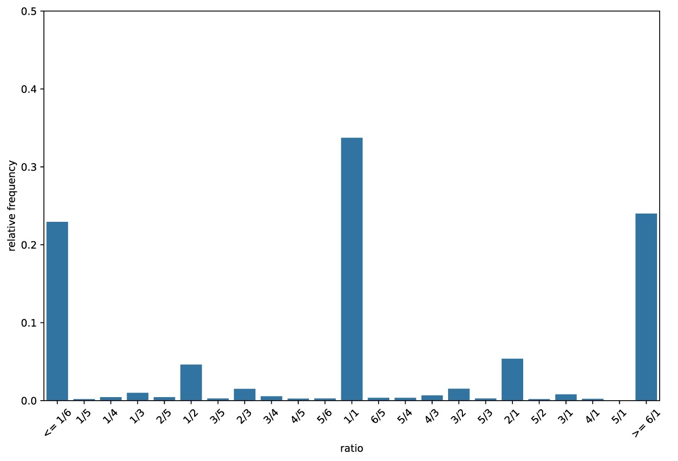
The Above plot was created from a query genome with 61% completeness and 30% contamination.
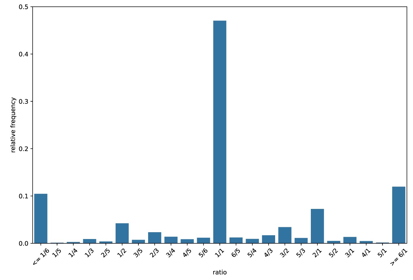
The Above plot was created from a query genome with 90% completeness and 10% contamination.
Machine learning
The machine learning step uses the CRHs of the query genomes to improve/refine the marker-based estimations from stage I.
Two neural networks are used in this prediction refinement step. One neural network is used to improve the completeness estimation and one neural network is used to improve the contamination estimation.
The neural network implementations are from sklearn.
If you are interested in how the machine learning step work please see the CoCoPyE publication: https://academic.oup.com/gigascience/article/doi/10.1093/gigascience/giae079/7841111
23.2 Mamba
Due to program version conflicts we will use the CoCoPyE conda environment for this section.
Open a new terminal and activate the CoCoPyE environment.
Ensure you are in the correct directory.
23.3 CoCoPyE: run

cocopye has one main command to predict bin quality: cocopye run.
Run the cocopye command (this will take a while):
Parameters

-t: Number of threads/cores/CPUs to utilise for the process.-i: Input directory containing the bins in FASTA format.-o: Output file (more info below).
Other options include:
--file-extensions: The allowed file extensions for input files within the input directory.- The default is
fasta,fna,fa. Our bin files produced fromMetaBAT2have the file extension/suffix of.faso the default works.
- The default is
-v: The output file verbosity.- Values are:
standard(default),extended, andfull. - More information on the output below.
- Values are:
23.4 CoCoPyE: output

As we have only used a subset of data the results are not very good. We'll therefore look at premade results. These premade results were produced using the entire K1 dataset. First you will need to copy them.
cd ~/7-Binning
mkdir K1_fullset
cd K1_fullset
ln -s /pub14/tea/nsc206/NEOF/Shotgun_metagenomics/binning/K1_fullset/* .
Now we can look at the results table that is in your current directory.
#Use tr to tranform commas (,) to tabs (\t)
#This makes it easier to visually parse the columns
cat cocopye_output.csv | tr "," "\t" | lessOutput columns when -v set to standard (also the default)
bin: Name of the input bin (filename excluding file extension)completeness: Completeness value between 0 and 1contamination: Contamination value between 0 and 1method: One of three results:- rejected: Failed the threshold in the input-preprocessing step.
- markers: Values based on stage I as failed to pass onto stage II due to the stage I thresholds
- markers + neural network: Values based on stage II as passed all thresholds
taxonomy: Taxonomy estimate based on a consensus between the nearest neighborstaxonomy_level: Rank of the taxonomy estimatenotes: Additional notes (currently this is always empty, but we might add some notes in the future)
Please see the full list of statistics definitions from CoCoPyE wiki. This includes the defintions when -v is set to extended or full.
23.5 CoCoPyE: Quality score

One quick way to calculate the overall quality of a bin is with the following equation:
\[ q = comp - (5 * cont) \] Where:
- q = Overall quality
- comp = Completeness
- cont = Contamination
A score of at least 70-80% (i.e. 0.7 to 0.8) would be the aim, with a maximum/perfect value being 100% (100% completeness, 0% contamination). Therefore let us calculate this for the bins with some bash and awk scripting.
Note: Values will range from:
- 100% (i.e. 1): 1 Completeness - (5 * 0 Contamination)
- -500% (i.e. -5): 0 Completeness - (5 * 1 Contamination)
Quality file
We will create a new file with only the quality information. We'll start by making a file with only a header.
Calculate quality with awk
Next is the most complicated command. We will be calculating the Overall quality (see calculation above) for each row except the header row.
We will be using a complicated linux based language called awk. This is very useful as it can carry out calculations on columns or as awk calls them, fields.
As this is new and complicated we will build up our command step by step.
Extract fields/columns
The first step is to extract the completeness and contamination fields/columns.
-F,: Indicates the input fields are separated by commas (,).'': All theawkoptions are contained within the quotes.{}: We can supply a function toawkwithin the braces.print $2,$3: This function instructsawkto print the 2nd (completeness) and 3rd (contamination) fields. It is common to put commas (,) between fields if printing multiple fields.cocopye_output.csv: Our last parameter is the input file. We are not changing the contents of the file, only printing information to screen/stdout.
Ignore header
We do not want the header in our calculation so we will add an extra awk option.
NR>1:NRstands for number of records. Rows are called records inawk. ThereforeNR>1meansawkwill only carry out the functions on the records numbered greater than 1. I.e. skip row 1, the header row.
Calculate quality
The next step is to carry out the overall quality calculation and append the information to the "MAGS_quality.csv" file.
Our new function, {print $2 - (5 * 13)}, carries out the overall quality calculation and prints it for each record/row except the first (NR>1).
You will notice that we have values that equal 4. Let us fix that.
Fix values
Some quality values come out as 4.
This is not correct and comes about as the completeness and contamination values have been set to -1 (-1 - (5 * -1) = 4).
If you look at the file cocopye_output.csv you will notice the bins with -1 values have the rejected for their method value.
These are bins which failed the Input Pre-procesing step.
We will therefore change these quality values to the lowest possible value of -5 (0 - (5 * 1) = -5).
In this case we pipe (|) our output to sed to substitute lines that start with (^) and end with ($) the same 4 with -5.
In other words we replace lines that only contain a 4 with a -5.
Append to quality file
Finally we can append the quality values to our MAGS_quality.csv file.
In the above case we use >> to append the information to the file MAGS_quality.csv. We append because we want to retain the header we added to the file earlier.
You can view the file to ensure it worked. The first and second values should be 0.9838 and 0.493
Add quality to the checkm results file
Now we can combine the files cocopye_output.csv and MAGS_quality.csv with the paste command into a new file called cocopye_quality.csv. The -d "," option indicates the merged files will be separated by commas (,), matching the column separation in cocopye_output.csv.
23.6 CheckM: MCQs

Viewing the file cocopye_output.csv attempt the below questions.
Tip: You can use the cut command to look at specific columns. For example:
#look at the "bin" and "quality" columns
#Convert the printed output's commas to tabs for readability
cut -d "," -f 1,8 cocopye_quality.csv | tr "," "\t"- What lineage was assigned to bin K1.1?
- What lineage was assigned to bin K1.22?
- What lineage was assigned to bin K1.8?
- What is the quality value of K1.1?
- What is the completeness value of K1.30?
- What is the contamination value of K1.12 bin?
- Which bin has the highest quality value (98.38%)?
- Which bin has the quality value of -2.9215?
- Which bin has the highest completeness value (98.59%)?
23.7 Bin quality summary

It is always useful to know the quality of your bins so you know which are more reliable than others. With that information you can be more or less certain when concluding your findings.
We have some good quality bins but many poorer quality bins too. Ultimately binning is trying to separate all the genomes from each other. A better metagenome assembly would most likely have led to better binning.