Chapter 7 Checking the quality of your data

Those of you who attended our Introduction to sequencing data and quality control course would have used FastQC to check the quality of the data. DADA2 has its own quality control option, which plots a similar read length by quality figure.
7.1 Forward read quality

To plot the quality of the forward reads:
- Import the cutadapt files
- Extract the sample names
- Run the
plotQualityProfilefunction
# Specify the paths and file names of the forward and reverse primer cleaned files
cutFs <- sort(list.files(path.cut, pattern = "_L001_R1_001.fastq", full.names = TRUE))
cutRs <- sort(list.files(path.cut, pattern = "_L001_R2_001.fastq", full.names = TRUE))

# Extract sample names
get.sample.name <- function(fname) strsplit(basename(fname), "_")[[1]][2]
sample.names <- unname(sapply(cutFs, get.sample.name))
head(sample.names)

# check the quality for the first file
plotQualityProfile(cutFs[1:1])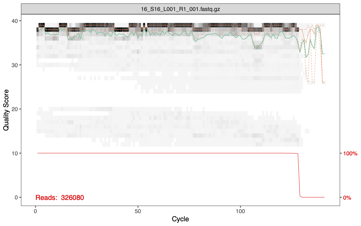
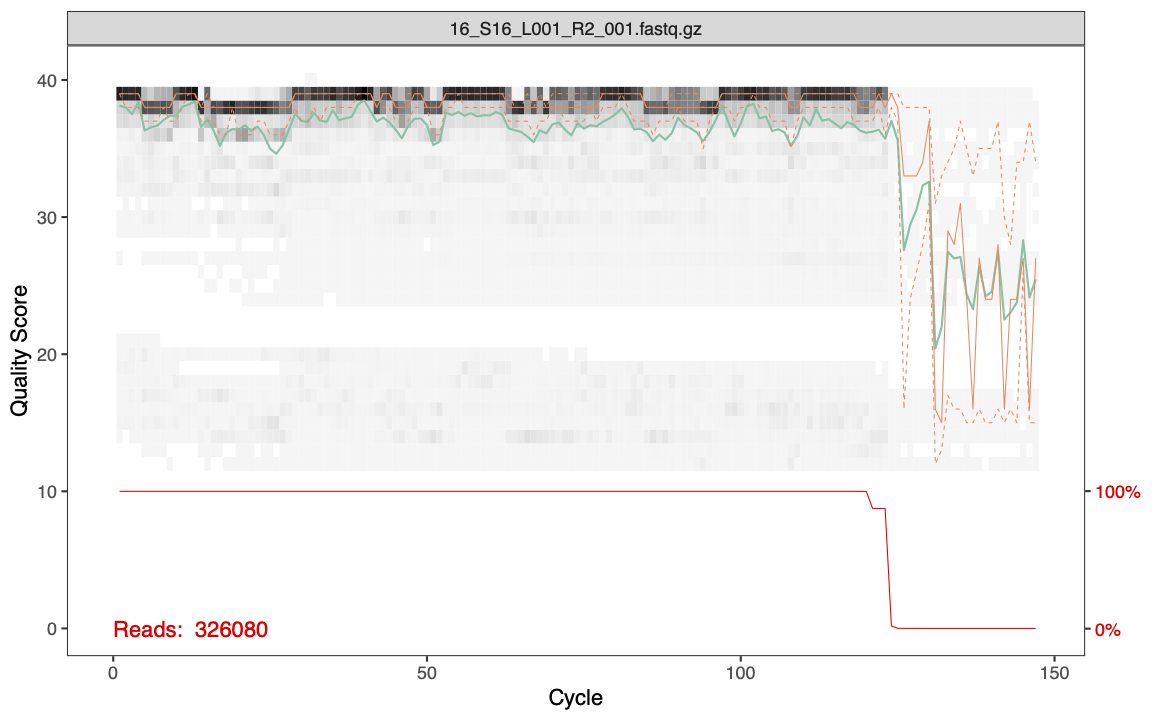
The features of the plot include:
- Gray-scale heatmap: Shows the frequency of each quality score along the forward read lengths
- Green line: The median quality score
- Orange lines: The quartiles
- Red line: Situated at the bottom of the plot, it represents the proportion of reads of that particular length.
- Its y-axis values are on the right side of the plot.
The quality is very good for our forward reads. You can also see that the majority of the forward reads are ~130bp long after having the primers removed with cutadapt.