Chapter 14 Plots exercises

These exercises will primarily use the "penguin_df" from the theory and practice session.
Please use your "Exercises.R" script for this exercise and the main workshop directory as the working directory. Ensure you are using annotations and code sections to keep the contents clear and separated.
For convenience the code to load the Penguin data frame directory will be:
penguin_df <- read.csv("Chapter_12-14/penguin.tsv",
                      check.names = FALSE,
                      stringsAsFactors = TRUE,
                      sep = "\t"
                      )
Your plots might not look exactly the same. As long as your plot contains the same data it is good.
Solutions are in the expandable boxes. Try your best to solve each challenge but use the solutions for help if you would like. Even if your method works it can be good to check the solution as there are many ways to do the same thing in R.
14.1 Line graph
First we will ignore "penguin_df".
Create the below plot. You will need to create the vectors yourself.
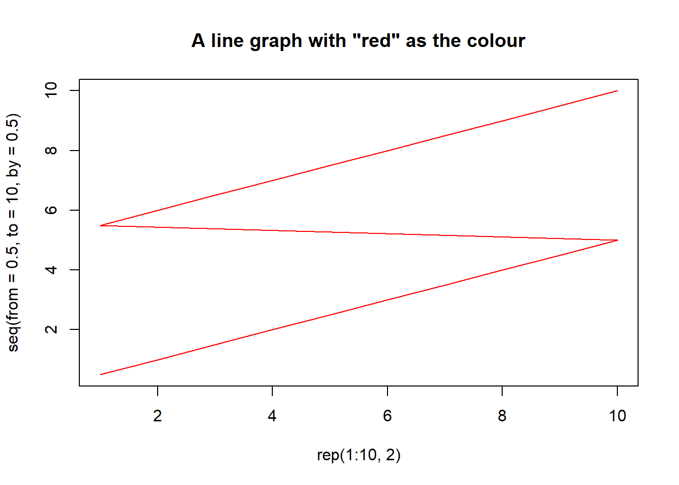
Tip: The x and y labels may help you figure out the commands to create the vectors.
14.2 Histogram
From the "penguin_df" create the below plot:
Note: The colour of the bars are "blue".
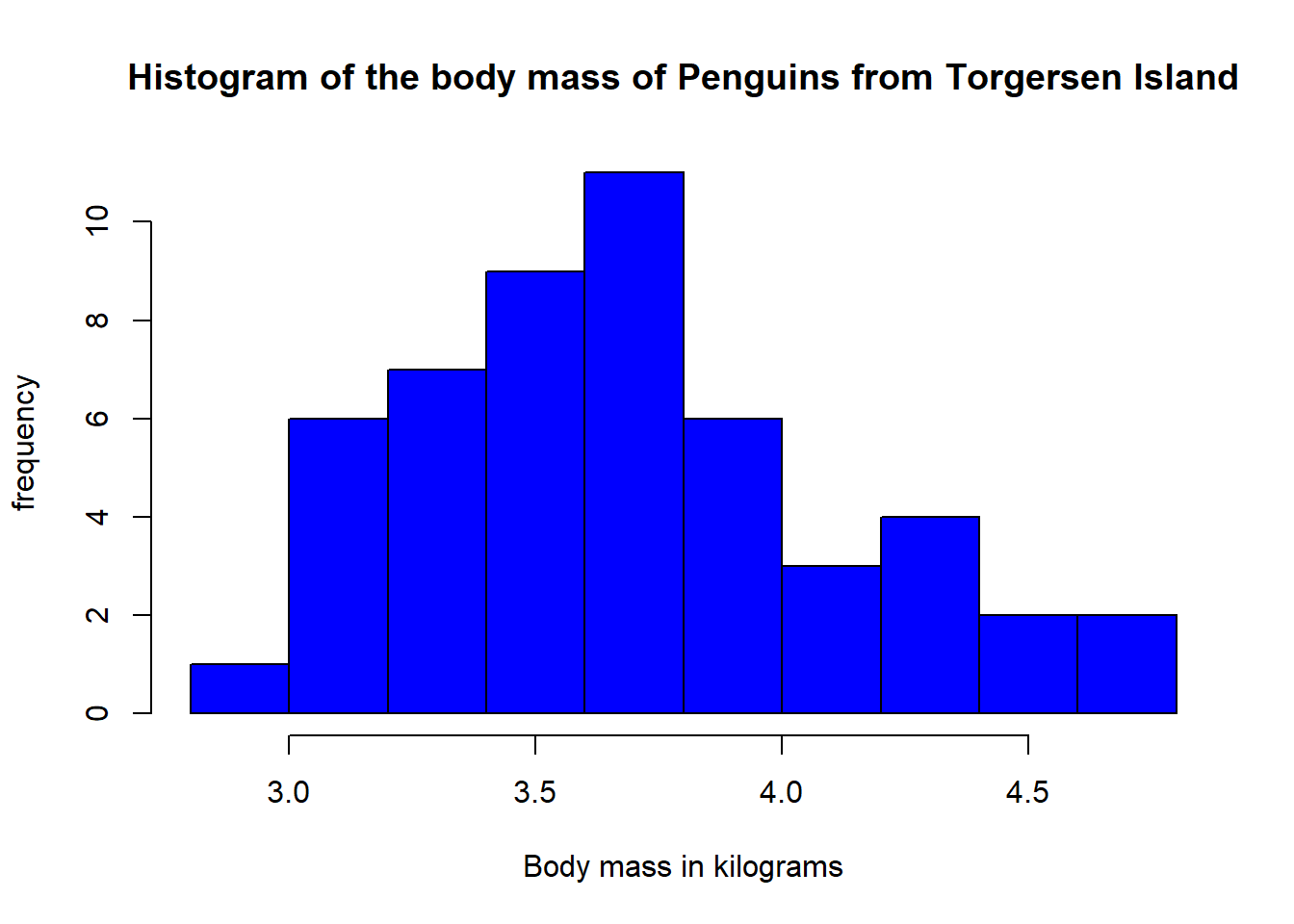
#Create data frame with only the Penguins from Torgersen
penguins_torgensen_df <- penguin_df[penguin_df$island == "Torgersen",]
#Create a column with body mass in kilograms
penguins_torgensen_df$body_mass_kg <-
penguins_torgensen_df$body_mass_g / 1000
#Plot the histogram
hist(penguins_torgensen_df$body_mass_kg,
main = "Histogram of the body mass of Penguins from Torgersen Island",
xlab = "Body mass in kilograms",
ylab = "frequency",
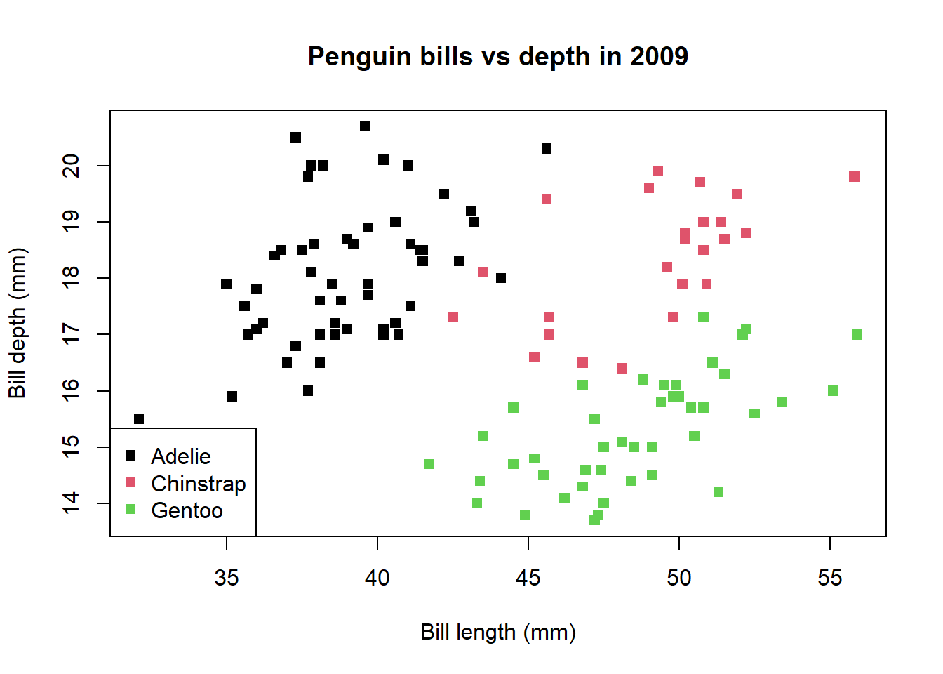
col = "blue")14.3 Scatterplot
From the "penguin_df" create the below plot:
Note: You can check what numbers refer to what shape for pch = at: http://www.sthda.com/english/wiki/r-plot-pch-symbols-the-different-point-shapes-available-in-r
Before you continue save this plot. Details below:
- Save the file as a png called "Penguins_2009_bill_depth_vs_length_scatterplot.png"
- Save the plot with a width and height of 250 and resolution of 150
#Create data frame with only the Penguins from 2009
penguin_2009_df <- penguin_df[penguin_df$year == "2009",]
#Start png function
png(filename = "Chapter_12-14/Penguins_2009_bill_depth_vs_length_scatterplot.png",
units = "mm", height = 250, width = 250, res = 150 )
#Produce plot
plot(x = penguin_2009_df$bill_length_mm,
y = penguin_2009_df$bill_depth_mm,
col = as.numeric(penguin_2009_df$species),
main = "Penguin bills vs depth in 2009",
xlab = "Bill length (mm)",
ylab = "Bill depth (mm)",
pch = 15)
#Create legend
legend(x = "bottomleft",
col = 1:nlevels(penguin_2009_df$species),
legend = levels(penguin_2009_df$species),
pch = 15)
#Save file
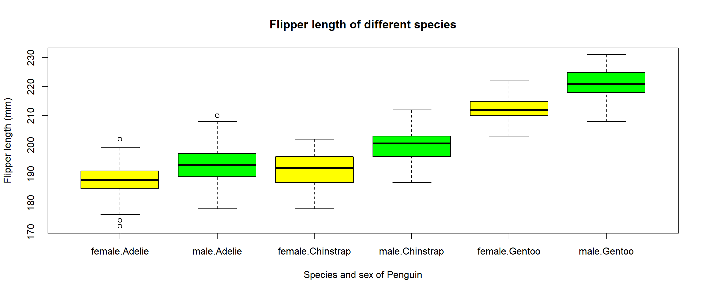
dev.off()14.4 Boxplot
From the "penguin_df" create the below plot:
Note: Make sure the x axis is in the same order as below.
For the last task, save this plot. Details below:
- Save the file as a jpg called "Penguins_species_and_flipper_length_boxplot.jpg" in "Chapter_12-14".
- Save the plot with a width of 300, height of 250, and resolution of 150
#Start png function
jpeg(filename = "Chapter_12-14/Penguins_species_and_flipper_length_boxplot.jpg",
    units = "mm", height = 250, width = 300, res = 150 )
#Produce boxplot
boxplot(flipper_length_mm~sex*species,
        data = penguin_df,
        col = c("yellow","green"),
        main = "Flipper length of different species",
        xlab = "Species and sex of Penguin",
        ylab = "Flipper length (mm)"
)
#Save file
dev.off()